Complexity and Networks
The Kuramoto model - Part II
Konstantinos Efstathiou

Linear stability of the incoherent state in the Kuramoto model
Continuum limit
The idea here is to consider the limit \(N \to \infty\) and express this by using distributions of oscillators instead of discrete oscillators. We denote by \[ \rho(\theta,t,\omega) \] the probability density that an oscillator of natural frequency \(\omega\) has phase \(\theta\) at time \(t\).
The normalization condition is that \[ \int_0^{2\pi} \rho(\theta,t,\omega) \, d\theta = 1. \]
Since the number of oscillators is conserved we can write a continuity equation which can be derived in the same way as the continuity equation for 1-dimensional fluids. The continuity equation is \[ \frac{\partial \rho}{\partial t} + \frac{\partial }{\partial \theta} (\rho \upsilon) = 0, \] where \(\upsilon\) is the velocity of an oscillator with natural frequency \(\omega\) and phase \(\theta\). Therefore, \[ \upsilon = \dot\theta = \omega + K r \sin (\psi - \theta). \]
The order parameter can be written in terms of these distributions as \[ r e^{i \psi} = \int_{0}^{2\pi} \int_{-\infty}^\infty \rho(\theta',t,\omega') g(\omega') e^{i\theta'} \,d\omega'\,d\theta'. \]
Therefore, \[ r e^{i (\psi-\theta)} = \int_{0}^{2\pi} \int_{-\infty}^\infty \rho(\theta',t,\omega') g(\omega') e^{i(\theta'-\theta)} \,d\omega'\,d\theta', \] and we finally obtain by considering the imaginary parts that \[ \upsilon = \omega + K \int_{0}^{2\pi} \int_{-\infty}^\infty \rho(\theta',t,\omega') g(\omega') \sin(\theta'-\theta) \,d\omega'\,d\theta'. \]
The full equation for the continuum limit of the Kuramoto model can then be written as
Stationary solutions
Stationary distributions do not change in time. Therefore, \(\partial\rho/\partial t=0\) and \[ \frac{\partial }{\partial \theta} (\rho \upsilon) = 0, \] implying \[ \rho \upsilon = C(\omega). \] If \(C(\omega) \ne 0\), then \(\rho = C(\omega)/\upsilon\). If \(C(\omega) = 0\) then \(\rho\) is a delta-function at \(\upsilon=0\).
A stationary distribution is the uniform distribution \[ \rho(\theta,\omega) = \frac{1}{2\pi}, \] which can be easily seen to satisfy the continuum limit Kuramoto equation and which corresponds to the incoherent state.
Perturbations of the incoherent state
Consider the perturbation of the incoherent state given by \[ \rho(\theta,t,\omega) = \frac{1}{2\pi} + \varepsilon \, \eta(\theta,t,\omega). \]
Exercise. Show that to first order in \(\varepsilon\) we have
We write a Fourier series for \(\eta\) as \[ \eta(\theta,t,\omega) = \sum_{n=1}^\infty c_n(t,\omega) e^{in\theta} + \bar{c}_n(t,\omega) e^{-in\theta}. \]
Then \[ \int_{0}^{2\pi} \eta(\theta',t,\omega') \sin(\theta'-\theta) \,d\theta' = -2 \pi \mathrm{Im}(c_1 e^{i\theta}). \]
Subsequently, we find that \[ \frac{\partial c_1}{\partial t} + i \omega c_1 - \frac{K}{2} \int_{-\infty}^\infty c_1(t,\omega') g(\omega') d\omega' = 0, \]
and, for \(n \ge 2\), \[ \frac{\partial c_n}{\partial t} + i n \omega c_n = 0. \]
Therefore, for \(n \ge 2\) we immediately obtain \[ c_n(t,\omega) = c_n(0,\omega) e^{i n \omega t}. \]
For \(n=1\) we consider the operator \(A\) given by \[ A c := - i \omega c + \frac{K}{2} \int_{-\infty}^\infty c(t,\omega') g(\omega') d\omega', \] so that we can write \[ \frac{\partial c_1}{\partial t} = A c_1. \]
It turns out that the spectrum of \(A\) has a continuous part given by \[ \{ i \omega : \omega \in \mathrm{supp}(g) \}. \] Such eigenvalues imply neutral stability. If we only have eigenvalues on the imaginary axis then the linear stability analysis is not sufficient to determine the stability of the solution.
We look for discrete eigenvalues of \(A\) through the ansatz \[ c(t,\omega) = b(\omega) e^{\lambda t}. \]
Then \[ \lambda b = - i \omega b + \frac{K}{2} \int_{-\infty}^\infty b(\omega') g(\omega') d\omega'. \] Let \[ B = \frac{K}{2} \int_{-\infty}^\infty b(\omega') g(\omega') d\omega'. \] Then \[ b(\omega) = \frac{B}{\lambda + i\omega}. \]
Therefore, we can write \[ \lambda \frac{B}{\lambda + i\omega} = - i \omega \frac{B}{\lambda + i\omega} + \frac{K}{2} \int_{-\infty}^\infty \frac{B}{\lambda+i\omega'} g(\omega') d\omega', \] implying \[ 1 = \frac{K}{2} \int_{-\infty}^\infty \frac{g(\omega')}{\lambda+i\omega'} d\omega'. \] We consider again a Lorentzian distribution \[ g(\omega) = \frac{\gamma}{\pi(\omega^2+\gamma^2)}. \] Therefore, \[ 1 = \frac{K}{2} \int_{-\infty}^\infty \frac{1}{\lambda+i\omega} \frac{\gamma}{\pi(\omega^2+\gamma^2)} d\omega = \frac{K\gamma}{2\pi i} \int_{-\infty}^\infty \frac{1}{\omega-i\lambda} \frac{1}{\omega^2+\gamma^2} d\omega. \]
Using residues we find (closing the integration path with a half-circle on the upper-half complex plane) that for \(\lambda < 0\) we have the contradiction \[ 1 = K \gamma \mathrm{Res}(i\gamma) = \frac{K}{2(\lambda-\gamma)} < 0. \] For \(\lambda > 0\) we find (closing the integration path with a half-circle on the lower-half complex plane) \[ 1 = - K \gamma \mathrm{Res}(-i\gamma) = \frac{K}{2(\lambda+\gamma)}, \] giving \[ \lambda = \frac{K}{2} - \gamma = \frac{K - K_c}{2}. \]
This shows that for \(K > K_c\) the incoherent state becomes unstable and small perturbations grow exponentially as \[ \sim e^{\frac{K-K_c}{2} t}. \]
Ott-Antonsen ansatz
The Ott-Antonsen ansatz is a method that allows to find the time evolution of \(r(t)\) (the modulus of the order parameter) for special types of solutions of the Kuramoto model.
Recall that the full equation for the continuum limit of the Kuramoto model has the form
\[ \frac{\partial \rho}{\partial t} + \frac{\partial }{\partial \theta} \left[\rho \left( \omega + K \int_{0}^{2\pi} \int_{-\infty}^\infty \rho(\theta',t,\omega') g(\omega') \sin(\theta'-\theta) \,d\omega'\,d\theta' \right)\right] = 0. \]
The left-hand side of the equation becomes
A Fourier series expansion of \(\rho\) gives \[ \rho(\theta,t,\omega) = \frac{1}{2\pi} \sum_{n=-\infty}^{\infty} c_n(t,\omega) e^{i n \theta}, \] where \(c_{-n} = \bar{c}_n\) and \(c_0 = 1\) (the last relation because of the normalization of \(\rho(\theta,t,\omega)\)).
Then we have \[\begin{align*} r e^{i\psi} &= \int_{-\infty}^\infty d\omega' g(\omega') \int_{0}^{2\pi} d\theta' \rho(\theta',t,\omega') e^{i\theta'} \\ &= \int_{-\infty}^\infty d\omega' g(\omega') \left( \frac{1}{2\pi} \sum_{n=-\infty}^\infty c_n(t,\omega') \int_{0}^{2\pi} d\theta' e^{in\theta'} e^{i\theta'} \right) \\ &= \int_{-\infty}^\infty d\omega' g(\omega') c_{-1}(t,\omega') = \int_{-\infty}^\infty d\omega' g(\omega') \bar{c}_{1}(t,\omega'). \end{align*}\]
Substituting the Fourier series for \(\rho\) into the equation \[\begin{align*} 0 &= \frac{\partial \rho}{\partial t} + \frac{\partial }{\partial \theta} \left[\rho \left( \omega + K \, \mathrm{Im} \left( r e^{i\psi} e^{-i\theta} \right)\right)\right] \\ &= \frac{\partial \rho}{\partial t} + \frac{\partial }{\partial \theta} \left[\rho \left( \omega + \frac{K}{2i} r e^{i\psi} e^{-i\theta} - \frac{K}{2i} r e^{-i\psi} e^{i\theta} \right)\right], \end{align*}\] we obtain the relation \[ \frac{\partial c_n}{\partial t} + in\left( \omega c_n + \frac{K r e^{i\psi}}{2i} c_{n+1} - \frac{Kr e^{-i\psi}}{2i} c_{n-1} \right) = 0. \]
The Ott-Antonsen ansatz is to consider distributions with \(c_n(t,\omega) = \alpha(t,\omega)^n\), for \(n \ge 1\). Consequently, \(c_{n} = \bar{c}_{|n|} = \bar{\alpha}^{|n|}\) for \(n \le -1\).
Then,
\[ r e^{-i\psi} = \int_{-\infty}^\infty d\omega' g(\omega') \alpha(t,\omega'), \]
and the equation for \(c_n\) from the previous slide becomes
\[ \frac{\partial \alpha}{\partial t} + i \omega \alpha + \frac{K r e^{-i\psi}}{2} [e^{2i\psi}\alpha^2 - 1] = 0. \]
We now compute the integral
\[ r e^{-i\psi} = \int_{-\infty}^\infty d\omega' g(\omega') \alpha(t,\omega'), \]
assuming that \(\alpha\) is analytic in the lower half complex plane (as a function of a complexified \(\omega\)).
Then, choosing a Lorentzian \(g(\omega) = \gamma/(\pi(\omega^2+\gamma^2))\) we have
\[ r e^{-i\psi} = \int_{-\infty}^\infty d\omega' g(\omega') \alpha(t,\omega') = - 2\pi i \mathrm{Res}(-i\gamma) = \alpha(-i\gamma,t). \]
Setting \(\omega=-i\gamma\) into the equation for \(\alpha\) and using the relation between the order parameter and \(\alpha(-i\gamma,t)\) we obtain
\[ \frac{d}{dt}(r e^{-i\psi}) + \gamma r e^{-i\psi} + \frac{K r e^{-i\psi}}{2} [r^2-1] = 0. \]
Then \[ \frac{dr}{dt}e^{-i\psi} - ir \frac{d\psi}{dt}e^{-i\psi} + \gamma r e^{-i\psi} + \frac{K r e^{-i\psi}}{2} [r^2-1] = 0, \] and \[ \frac{dr}{dt} - ir \frac{d\psi}{dt} + \gamma r + \frac{K r}{2} [r^2-1] = 0. \]
Therefore, we get two equations. The first one is \(r \dot\psi = 0\) and the second one is \[ \frac{dr}{dt} + \gamma r + \frac{K r}{2} [r^2-1] = 0. \]
The equation \[ \frac{dr}{dt} + \gamma r + \frac{K r}{2} (r^2-1) = 0. \] has equilbria \(r = 0\) and \(r = \sqrt{1-K_c/K}\). These can be found by solving the equation \[ f(r) = - \gamma r - \frac{K r}{2} (r^2-1) = 0. \]
For the linear stability we need to consider the linearization at the equilibria. This can be determined through the derivative at the equilibria. We have \[ f'(r) = -\gamma + \frac{K}{2} - \frac{3 K r^2}{2}. \]
For the incoherent state, \(r = 0\), we get \[ f'(0) = -\gamma+\frac{K}{2} = \frac{K-K_c}{2}, \] where \(K_c=2\gamma\).
Therefore the incoherent state seems be stable if \(f'(0) < 0\) which implies \(K < K_c\), and unstable if \(K > K_c\).
For the second branch, given by \(r = r_* = \sqrt{1-K/K_c}\) for \(K > K_c\), we have
\[ f'(r_*) = -(K - K_c). \]
Therefore, this branch is stable for \(K > K_c\) (and it does not exist for \(K<K_c\)).
The equation for \(r\), \[ \frac{dr}{dt} + \gamma r + \frac{K r}{2} (r^2-1) = 0, \] is separable and can be easily integrated. Nevertheless, the computations become easier making the substitution \(u = r^2\) which gives \(\dot{u} = 2 r \dot{r}\). Multiplying the previous equation by \(2r\) we find \[ 2 r \frac{dr}{dt} + 2 \gamma r^2 + K r^2 (r^2-1) = 0, \] which becomes \[ \frac{du}{dt} = - K_c u - K u (u-1). \] Rearranging terms we find \[ \frac{du}{dt} = (K-K_c) u - K u^2, \]
and \[ \frac{du}{K dt} = \left(1-\frac{K_c}{K}\right) u - u^2. \] Let \[ \delta = 1-\frac{K_c}{K}. \] Then the equation becomes \[ \frac{du}{K dt} = \delta u - u^2, \] which is a rewriting of the logistic equation.
Integration gives
\[ \frac{1}{\delta} \ln \left| \frac{u}{u-\delta} \right| = K t, \] and then \[ \frac{u}{u-\delta} = A e^{\delta K t} = A e^{(K-K_c)t}. \]
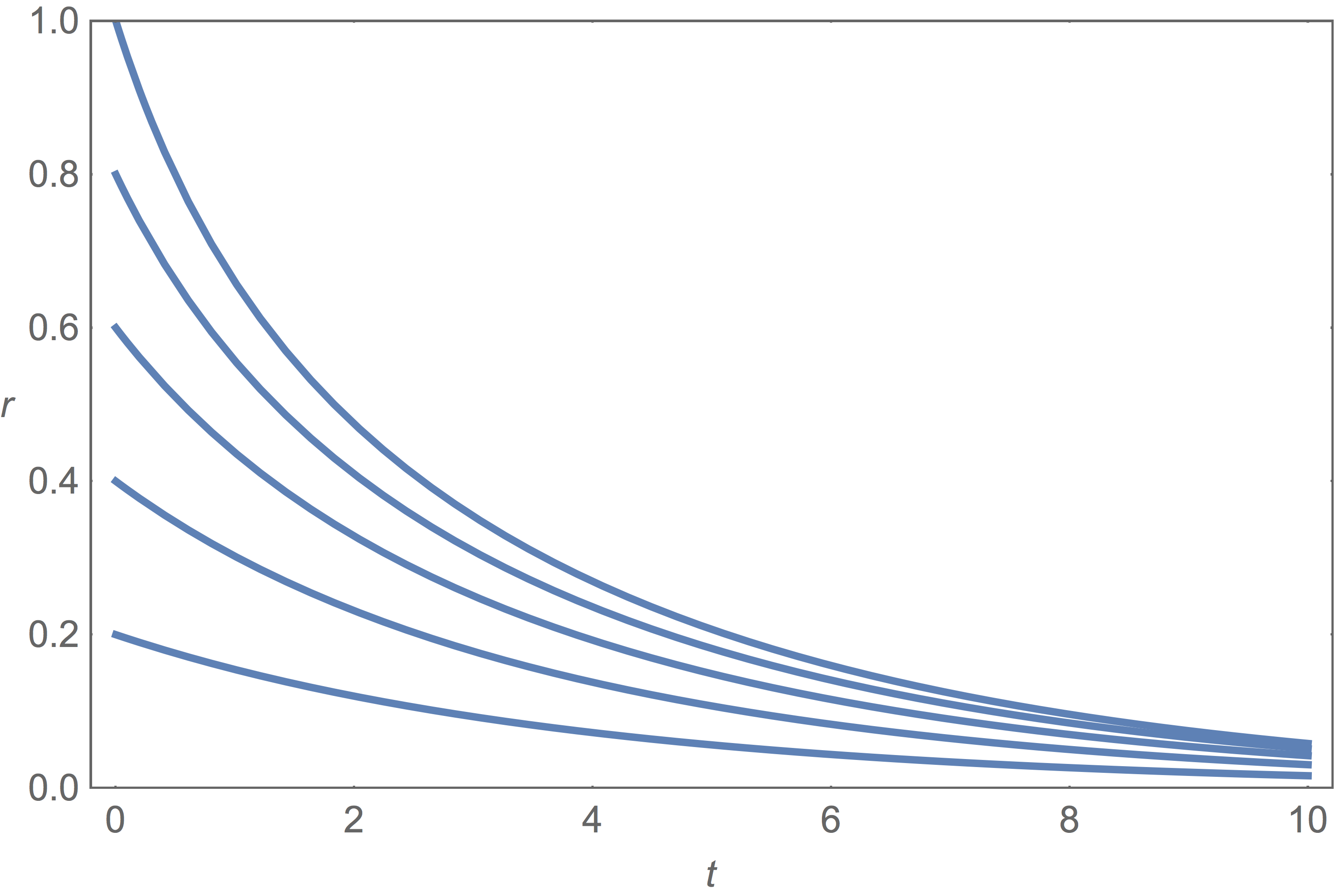
Solving for \(u\) we find \[ u = \frac{\delta}{1-\frac{1}{A} e^{-(K-K_c) t}}. \] Moreover, if for \(t=0\) we have \(u=u_0\) we can write \[ A = \frac{u_0}{u_0-\delta}, \] and we get \[ u = \frac{\delta u_0}{u_0 - (u_0-\delta) e^{-(K-K_c) t}}. \]
For \(t \to \infty\) we find that if \(K - K_c < 0\) then \(u \to 0\).
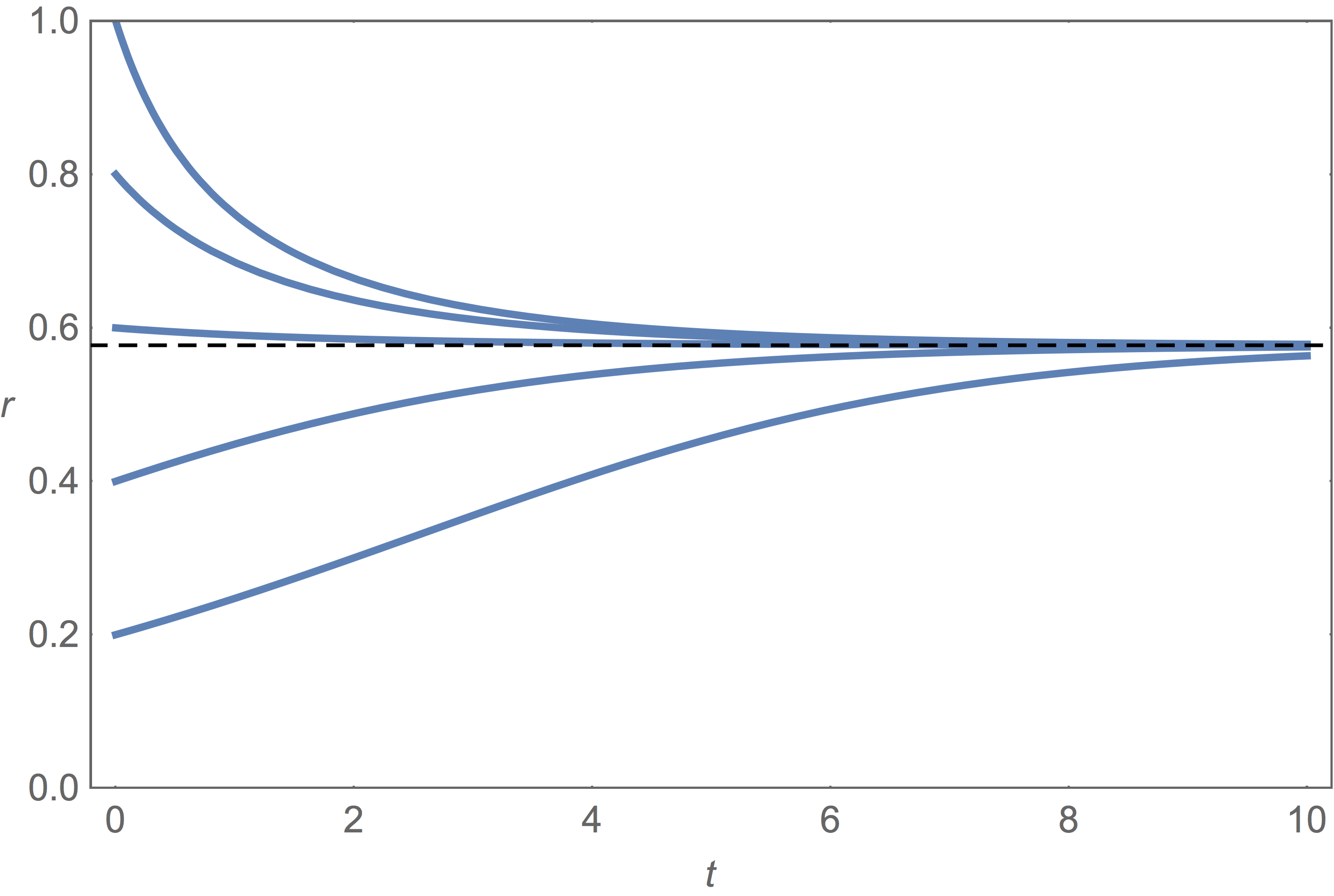
If \(K \delta > 0\) and \(u_0 \ne 0\) then for \(t \to \infty\) we find \(u \to \delta\), implying \[ r \to \sqrt{1-\frac{K_c}{K}}. \] Finally, if \(u_0 = 0\) then \(u = 0\) for all \(t\).