Until now we have been considering oscillators that are connected all-to-all and in the same way. Now we will consider networks where each node is connected to some other nodes but possibly (and typically) not all.

In mathematics, a network is often called a graph. The network nodes are called vertices and the network connections are called edges.

Adjacency matrix

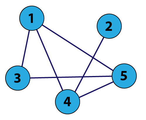
The network structure is described through the adjacency matrix A=(aij). This is defined by

aij={1, if node i is connected to node j, 0, otherwise. 

Clearly, A is a real symmetric matrix, that is, At=A.

Example

Node degree

The degree ki of the i-th node is defined as the number of nodes that are directly connected to the i-th node. It follows that

ki=n∑j=1aij.

The average degree is

⟨k⟩=1nn∑i=1ki=1nn∑i=1n∑j=1aij.

The degree matrix is

D=diag(k1,k2,…,kn).

Example

Graph Laplacian

The graph Laplacian is defined by

L=D−A,

that is,

Lij=kiδij−aij.

L is a real symmetric matrix and this implies that it has real eigenvalues.

Moreover, it is possible to show that L is positive semidefinite, that is,

xtLx≥0,

for all x∈Rn.

This implies that the eigenvalues of L are non-negative.

Exercise. Show that xtLx=12n∑i,j=1aij(xi−xj)2.

Example

Eigenvalues of the graph Laplacian

The eigenvalues of L are

0=λ1≤λ2≤⋯≤λn≤n.

To show that 0 is always an eigenvalue consider the vector 1=(1,…,1)t.

Then

(L1)j=n∑i=1Lji1i=n∑i=1Lji=n∑i=1kjδji−aji=kj−n∑i=1aji=kj−kj=0.

Therefore,

L1=0=01,

implying that 0 is an eigenvalue.

Exercise. Show that the number of zero eigenvalues of L gives the number of connected components of the network.

Complete graph

A complete graph is a graph in which all vertices are connected to all other vertices. In this case

λ2=⋯=λn=n.

One way to see this is to write

L=nI−C(1),

where C(1) is the n×n matrix with all entries equal to 1.

Then notice that any vector v with ∑ivi=0 is an eigenvector of C(1) with eigenvalue 0. Let Z be the set of all such vectors v. It can be easily shown that this is a vector subspace of Rn with dimension n−1.

Moreover, if v∈Z then

Lv=nv−C(1)v=nv.

Therefore, all v∈Z are eigenvectors of L with eigenvalue n and this implies that n must be an eigenvalue of L with mulitplicity n−1 (the same as the dimension of Z).

A basis of Z is given by the n−1 vectors
(1,−1,0,0,0,…,0),
(1,0,−1,0,0,…,0),
(1,0,0,−1,0,…,0),
…,
(1,0,0,0,0,…,−1).

Exercise. Construct an orthogonal basis of Z.

Example

Consider on a connected network the dynamical system

˙xi=Cn∑j=1aij(xj−xi),

where A=(aij) is the adjacency matrix. Such a system describes a diffusion process on the network.

Then

˙xi=Cn∑j=1aijxj−Cn∑j=1aijxi=Cn∑j=1aijxj−Ckixi.

Therefore,

˙x=CAx−CDx=−CLx.

This is a linear dynamical system. Its stability is determined by the eigenvalues of −CL.

If we denote by 0=λ1<λ2≤⋯≤λn the eigenvalues of L then the eigenvalues of −CL are 0=−Cλ1>−Cλ2≥⋯≥−Cλn. In particular, all eigenvalues are strictly negative except for a single zero eigenvalue.

Let vi denote the corresponding eigenvectors, with v1=1. These are orthogonal. We have x(t)=n∑i=1ci(t)vi and then ˙x(t)=n∑i=1˙ci(t)vi=−CLn∑i=1ci(t)vi=−Cn∑i=1ci(t)λivi.

From here we get

˙ci=−Cλici,

with solution

ci(t)=e−Cλitci(0).

This means

x(t)=n∑i=1e−Cλitci(0)vit→∞⟶c1(0)1,

where we used that λ1=0 and v1=1.

We consider now a network where each node has dynamics given by the equation

˙xi=f(xi)

where xi∈Rk and f:Rk→Rk. In particular, and unlike the Kuramoto model where we assumed that the natural frequencies of the oscillators were not the same, here we assume that each node has identical dynamics.

Then we introduce the coupling between nodes as

˙xi=f(xi)+ϵn∑j=1aij(h(xj)−h(xi))=f(xi)−ϵn∑j=1Lijh(xj),

where L is the graph Laplacian and h:Rk→Rk is a given function.

It is easy to see that there exists a completely synchronized solution

x1(t)=x2(t)=⋯=xn(t)=s(t),

since in that case the coupling terms vanish and all oscillators satisfy the equations

˙s=f(s).

Our aim is to characterize the linear stability of the synchronized solution.

Linear stability of synchronized solution

As usual we consider a small deviation from the synchronized solution, that is, we write

xi(t)=s(t)+ξi(t).

Then we get the linearized equations of motion

˙ξi=Df(s)ξi−ϵn∑j=1LijDh(s)ξj=Df(s)ξi−ϵDh(s)n∑j=1Lijξj.

Notice that this is a time-dependent equation since s=s(t).

Write ξ for the k×n matrix given by

ξ=(ξ1,…,ξn)

and write

ξ=ζ1vt1+⋯+ζnvtn=n∑j=1ζjvtj,

where v1,…,vn are the eigenvectors of L, and ζ1,…,ζn∈Rk are time-dependent vector coefficients.

The equations from the previous slide can be collectively written as

˙ξ=Df(s)ξ−ϵDh(s)ξLt.

Then substitution gives

n∑j=1˙ζjvtj=n∑j=1[Df(s)ζj−ϵλjDh(s)ζj]vtj,

where we used that vtjLt=(Lvj)t=λjvtj.

From the last equation we obtain ˙ζj=[Df(s)−ϵλjDh(s)]ζj,

Therefore we see that along each eigenmode of L, given by vj, the linearized equations have the same form ˙ζ=[Df(s)−γDh(s)]ζ, where γ=ϵλj for ζ=ζj.

We write the previous equation in the form

˙ζ=A(t)ζ,

where A(t)=Df(s(t))−γDh(s(t)).

Moreover, we will assume here that the synchronized solution s(t) is a periodic orbit in Rk, that is, there is some T>0 such that s(t+T)=s(t) for all t∈R.

Floquet theory

We will now discuss (in general) the equation

˙v=A(t)v,

where, with the assumption that s has period T, we have A(t+T)=A(t).

If at t=0 we have v=v(0) then after time T we will have the vector v(T) by solving the equation ˙v=A(t)v. This defines a linear mapping

v(0)↦v(T)

which can be expressed in terms of a matrix M, called the monodromy matrix.

This allows us to describe the dynamics and its stability through the mapping v↦Mv. In particular, the stability of ˙v=Av will correspond to stability of v↦Mv.

The eigenvalues of M are called characteristic multipliers.

The Floquet exponents are defined by eμT=λ where λ are characteristic multipliers.

Finally, the Lyapunov exponents in this context are defined as Re(μ).

The reason that these are important is because of the following stability classification of v↦Mv. Let λi be the eigenvalues of M (characteristic multipliers). Then

• If all |λi|<1 then the map is asymptotically stable. This follows from the fact v=∑ni=1civi after k iterations of the map goes to Mkv=∑ni=1λkicivi and in this case λki→0 as k→∞.

• If there is some |λj|>1 then the map is unstable. This follows from the observation that if v=vj then Mkv=λkjvj and in this case λkj→∞ as k→∞.

If we write as α the Lyapunov exponent corresponding to λ then we have e(α+iβ)T=λ, so |λ|=eαT.

Therefore, we can say that

• If all αi<0 then the map is asymptotically stable.

• If there is some αj>0 then the map is unstable.

Master stability function

Recall that here we consider the linear system

˙ζ=A(t)ζ=[Df(s(t))−γDh(s(t))]ζ

The master stability function is the function g(γ) that assigns to γ the corresponding maximal Lyapunov exponent of the system above.

Suppose that g(γ)<0 for γmin<γ<γmax. Then the system is linearly stable if

γmin<ϵλ2≤ϵλn<γmax,

that is, if all eigenmodes give negative maximal Lyapunov exponent.

The region of the coupling strength for which the synchronized solution is stable is then

γminλ2<ϵ<γmaxλn.

This implies that in order for such an interval to be non-empty we must have

R:=λnλ2<γmaxγmin.

Notice that R depends only on the network topology (its graph Laplacian) while the master stability function (and subsequently γmin and γmax) depends only on the dynamics.

Therefore, the master stability formalism allows us to decouple the topology from the dynamics. After computing the master stability function for some coupling we can then find the eigenvalues of the graph Laplacian and determine which topologies are the most “synchronizable”.

Finally, suppose that g(γ)<0 for γmin<γ. Then the system is linearly stable if

γmin<ϵλ2.

This means that there is always in this case a value

ϵc=γminλ2,

such that if ϵ>ϵc then the synchronized solution is stable.