Remark. This lecture is based on Pacer cell response to periodic zeitgebers. D.G.M. Beersma, H.W. Broer, K. Efstathiou, K.A. Gargar, and I. Hoveijn. Physica D, 240:1516–1527 (2011).
The circadian clock resides in the suprachiasmatic nucleus, a neuronal hypothalamic tissue residing just above the optic chiasm. It consists of about 10000 interconnected neurons or pacer cells.
Each pacer cell is considered as a two-state (active-inactive) phase oscillator, where the phase is determined by a single variable \(\theta\) taking values in \([0,\tau]\).
In an isolated pacer cell the phase increases in time with speed 1 until it reaches a value \(\tau\); then it jumps to zero and starts to increase again.
The two states of the pacer cell are characterized as follows. If the phase is between zero and a value \(\alpha < \tau\), the cell is in the active state, and for the phase between \(\alpha\) and \(\tau\), the cell is in the inactive state. Thus an isolated pacer cell shows a periodic activity–inactivity cycle with period \(\tau\). We call \(\alpha\) the length of the intrinsic activity interval, and \(\tau\) is called the intrinsic period of the pacer cell.
In the active state, an external stimulus delays the phase and so the activity interval is prolonged. Suppose that at \(t = t_n\) the phase is zero. When the cell is stimulated by a Zeitgeber \(Z\), it remains active until time \(t_n + \alpha + \varepsilon Z\). This is achieved in the model by delaying the phase once by an amount of \(\epsilon Z\) at time \(t_n + \alpha\), so instantly \(\theta\) becomes \(\theta - \epsilon Z\).
In the inactive state, an external stimulus advances the phase and as a consequence the inactivity interval is shortened. If at time \(t = t_{n+1}\) the phase of the cell is below \(\tau\) by an amount \(\eta Z\), and so \(\theta + \eta Z = \tau\), the cell becomes active again. Thus there is a phase advance of \(\theta\) by an amount \(\eta Z\) at time \(t_{n+1}\); that is, instantly \(\theta\) becomes \(\theta + \eta Z\). Since the latter is equal to \(\tau\), the phase jumps to zero, and the cell is again in the active state.
The interaction of the pacer cells is by stimulation via the average of the activity of other pacer cells and by external stimuli such as light.
To understand synchronization properties we check how a single pacer cell interacts with the internal and external stimuli. This is reminiscent of the mean field approach in the Kuramoto model. We represent the effect of both types of stimuli through a function \(Z\) called Zeitgeber.
The Zeitgeber \(Z\) for the pacer cell singled out can be any function of time. Here we take it periodic, where the period is for example 24 hours, the period of the daily light and dark cycle. But we may also take a much longer period to model seasonal effects.
Since pacer cells may have different values of \(\epsilon\), \(\eta\), \(\alpha\) and \(\tau\) we are especially interested in the domain in parameter space where synchronization occurs.
Mathematical model
Each pacer cell is considered as a free running oscillator, depending on two parameters \(\alpha\), \(\tau\). The state of the pacer cell is determined by two variables: the phase\(\theta\) and the activity index\(a \in \{0,1\}\) taking the value \(0\) when the cell is inactive and \(1\) when it is active.
If the pacer cell is isolated (not coupled to any other pacer cell or external influence) then the phase increases with \(\dot\theta = 1\). Then \[\theta(t) = \theta(0) + t \pmod{\tau}.\] The activity index changes value from \(0\) to \(1\) when \(\theta(t)\) reaches the value \(\tau\) and continues from \(0\). It changes value from \(1\) to \(0\) when \(\theta(t)\) crosses the value \(\alpha\).
The Zeitgeber is given by a function \[
Z : \mathbb{R} \to [0,1]
\] which is assumed to be differentiable and periodic with period \(1\).
The coupling of the pacer cell to the Zeitgeber is now determined by the following rules. When \(\theta\) reaches the value \(\alpha\) at a time \(t\) the phase instantly drops by \(\epsilon Z(t)\). When the phase at a moment \(t_{n+1}\) reaches a value so that \[\theta(t_{n+1}) + \eta Z(t_{n+1}) = \tau\] then the phase instantly increases to \(\tau\). The moment \(t_{n+1}\) is defined implicitly by solving the equation above.
Dynamical system
We define a dynamical system on \(\mathbb{R}\) by computing the mapping \(t_n \mapsto t_{n+1}\) for the given dynamics. Here \(\{t_n\}\) is the set of transition times where the phase \(\theta\) reaches \(\tau\) and is subsequently reset to \(0\).
Actually, the “traditional” approach here would be, since we have a periodic Zeitgeber with period \(1\), to determine the mapping that gives the pacer cell phase at moments \(t \in \mathbb{Z}\), that is, \(\theta(n) \mapsto \theta(n+1)\).
From the map \(t_n \mapsto t_{n+1}\) we can see that a pacer cell synchronizes to the Zeitgeber (for example, daily light-dark cycle) if \(t_{n+1} = t_n + 1\).
Let \[
U_\epsilon(t) = t + \epsilon Z(t).
\]
Then the map that sends the transition time \(t_n\) to the next transition time \(t_{n+1}\) is given by \[
t_{n+1} = F_\mu(t_n) = U_\eta^{-1}(U_\epsilon(t_n+\alpha)-\alpha+\tau),
\] where \(\mu = (\epsilon,\eta,\alpha,\tau)\).
Proof
Let \(t_n\) be a transition time. Then at time \(t_n + \alpha\) the pacer cell reaches the value \(\alpha\) and its phase drops to \(\alpha - \epsilon Z(t_n + \alpha)\). From there the phase increases for time \(t_{n+1} - (t_n+\alpha)\) until it reaches a phase \[\begin{align*}
\theta
& = [\alpha - \epsilon Z(t_n + \alpha)] + [t_{n+1} - (t_n+\alpha)] \\
& = \alpha + t_{n+1} - [(t_n+\alpha) + \epsilon Z(t_n + \alpha)] \\
& = \alpha + t_{n+1} - U_\epsilon(t_n+\alpha),
\end{align*}\] such that \[
\theta + \eta Z(t_{n+1}) = \tau.
\]
Combining these two relations we find \[
\alpha + U_\eta(t_{n+1}) - U_\epsilon(t_n+\alpha) = \tau,
\] and \[
U_\eta(t_{n+1}) = U_\epsilon(t_n+\alpha) + \tau - \alpha.
\] If \(U_\eta\) has an inverse we reach the required relation for \(t_{n+1}\).
Analysis of the dynamics
Notice that \[
U_\epsilon(t+1) = t+1 + \epsilon Z(t+1)
= t + \epsilon Z(t) + 1 = U_\epsilon(t) + 1.
\] Moreover, if \(U_\epsilon\) has an inverse we get (replace \(t\) by \(U^{-1}(t)\) in the equation above) \[
U_\epsilon^{-1}(t+1) = U_\epsilon^{-1}(t) + 1.
\] Then \[\begin{align*}
F_\mu(t + 1)
& = U_\eta^{-1}(U_\epsilon(t+\alpha+1)-\alpha+\tau) \\
& = U_\eta^{-1}(U_\epsilon(t+\alpha)-\alpha+\tau + 1) \\
& = F_\mu(t) + 1.
\end{align*}\]
The relation \(F_\mu(t + 1) = F_\mu(t) + 1\) implies that there is a circle map\(f_\mu : \mathbb{S}^1 \to \mathbb{S}^1\) such that \(F_\mu\) is the lift of \(f_\mu\). By definition this means
If \(\rho\) is (sufficiently) irrational, then there is a change of coordinates \(t \mapsto x\) on the circle so that the map \(f\) becomes \(f(x) = x + \rho\).
If \(\rho\) is rational, that is, \(\rho = p/q\), then there exists an asymptotically stable period-\(q\) point \(t_*\) on the circle such that \(F^q(t_*) = t_*+p\).
We are interested in period-\(1\) points with \(F(t_*) = t_*+1\), that is, we want to find where \(\rho = 1\).
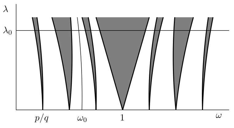
Typical picture of Arnol’d tongues for a circle map of the form \(f(t) = t + \omega + \lambda h(t)\). Each tongue represents a parameter region where the dynamics is “locked” to the rational \(p/q\).
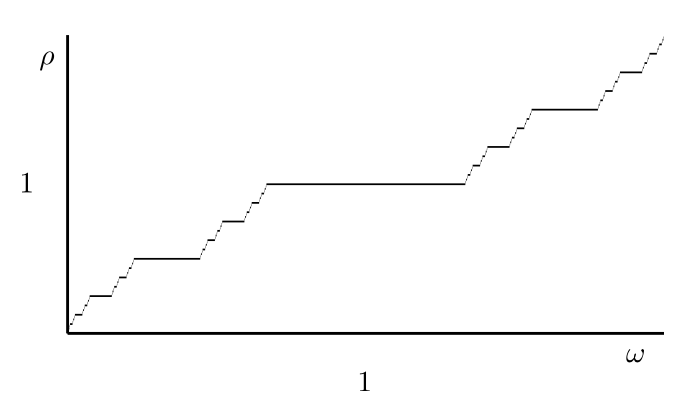
Typical dependence of the rotation number on \(\omega\) for a circle map of the form \(f(t) = t + \omega + \lambda h(t)\).
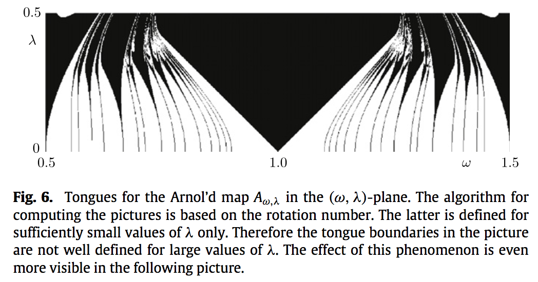
The Arnol’d circle map
The Arnol’d circle map, also known as sine-circle map, is defined by \[
A_{\omega,\lambda}(t) = t + \omega + \lambda \sin(2\pi t).
\]
It is a prototype for the dynamical behavior of circle maps.
Here we do not want to describe all the dynamics but only find those points for which \[
A_{\omega,\lambda}(t) = t + 1,
\] and correspond to periodic solutions with period \(1\).
We solve \[
t + \omega + \lambda \sin(2\pi t) = t + 1,
\] to find \[
\sin(2\pi t) = \frac{1-\omega}{\lambda}.
\] This equation has solutions only if \(|(1-\omega)/\lambda| \le 1\). There are two distinct solutions if \[
|1-\omega| < \lambda.
\] This is the region in the \((\omega,\lambda)\)-plane that lies between the lines \[\lambda = \pm(1-\omega).\]
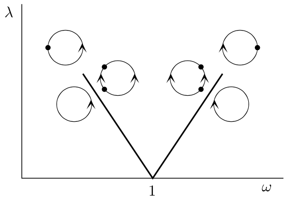
Main tongue for the Arnol’d map.
To find the stability of these two periodic points we do a linear stability analysis. Let \(t_*\) be any solution of \[
A_{\omega,\lambda}(t) = t + 1.
\] Then write \(t = t_* + s\). We get \[\begin{align*}
A_{\omega,\lambda}(t_*+s) & = t_* + s + \omega + \lambda \sin(2\pi (t_*+s)) \\
& = t_* + \omega + \lambda \sin(2\pi t_*) + s + 2\pi \lambda \cos(2\pi t_*) s \\
& = A_{\omega,\lambda}(t_*) + [1 + 2\pi \lambda \cos(2\pi t_*)] s \\
& = t_* + 1 + [1 + 2\pi \lambda \cos(2\pi t_*)] s.
\end{align*}\] This means that the map \(A_{\omega,\lambda}(t)\) induces the linear map \[
s \mapsto [1 + 2\pi \lambda \cos(2\pi t_*)] s,
\] at the fixed points.
The stability then depends on whether the absolute value of \[
a(t_*) := 1 + 2\pi \lambda \cos(2\pi t_*)
\] is larger than \(1\) (and we have instability) or smaller than \(1\) (and we have asymptotic stability).
For \(0 \le \lambda < 1/\pi\) there will always be one solution \(t_*\) for which \(|a(t_*)| < 1\) and one for which \(|a(t_*)| > 1\).
Remark. The condition \(\lambda < 1/\pi\) is natural, in the sense that it corresponds to the case where \(A_{\omega,\lambda}(t)\) is a diffeomorphism (in particular, it has an inverse).
Standard form of a circle map
Given the circle map \(F_\mu\) we can write \[
F_{\mu}(t) = t + \omega(\mu) + \lambda(\mu) R_\mu(t),
\] where \(\omega\) and \(\lambda\) depend on \(\mu\) and \(R_\mu(t)\) is a 1-periodic function with zero average.
Therefore, considering circle maps in the standard form is sufficient for our analysis although one has to consider how the initial parameters \(\mu=(\epsilon,\eta,\alpha,\tau)\) are mapped to the parameters \(\omega\) and \(\lambda\) of the standard form.
Special cases
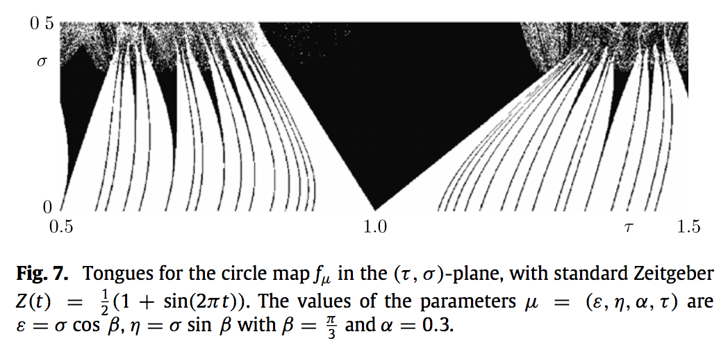
We introduce and from now on we use the standard Zeitgeber
\[
Z(t) = \frac12 (1 + \sin(2 \pi t)).
\]
Then we have that
\(F_{(\epsilon,0,\alpha,\tau)}\) is equivalent to \(A_{\tau+\epsilon/2,\epsilon/2}\) through a coordinate transformation that is a translation on the circle by \(\alpha\).
Here it is not easy to proceed the same way as for the Arnol’d circle map. Nevertheless, we can find the boundaries of the main tongue by noticing that there \(g(t)\) must have a double solution, implying that also \(g'(t) = 0\).
Therefore, we are interesting in finding the value of \(\tau\) as a function of other parameters so that simultaneously \(g(t) = 0\) and